2 Transport Processes
2.1 Diffusion Without Shear
(i) Instantaneous plane source in 3-dimensions
Suppose that the initial distribution of  is dependent only on
  and
and
 and that
  ,
,  and
and  are constant. Then Eq. (14) reduces to
We now transform to a frame of reference moving with the flow speed :
Then Eq. (15) becomes
Suppose that
 is constant. Then the solution to Eq. (16) is
It can be shown that
The solution (17) can
be interpreted as an instantaneous release of an amount  kgm
kgm of
pollutant at
of
pollutant at  in the plane
  . Eq. (17) is the Gaussian ``puff''
solution because it describes the release of a small ``puff'' of pollutant.
. Eq. (17) is the Gaussian ``puff''
solution because it describes the release of a small ``puff'' of pollutant.
An important quantity is the mean square distance  which the
pollutant has spread from
which the
pollutant has spread from  . This is given by
Therefore
The pollutant therefore spreads at a rate proportional to  .
.
(ii) Instantaneous line source in 3-dimensions
In this case we assume that  so that the equation for
is
so that the equation for
is
As in the previous case we make the transformation  and also
let
and also
let  . Then
The solution is
It can be shown that
 and
and
 . Hence
(iii) Instantaneous point source in 3-dimensions
This is the most general and practical case where  .
The equation for is
.
The equation for is
We
could put  in line with the cases of plane and line sources but
it is difficult to think of real cases where there is a mean vertical velocity
so we keep
in line with the cases of plane and line sources but
it is difficult to think of real cases where there is a mean vertical velocity
so we keep  . The transsformed equation for is then
The solution is
In this case
,
and
 so that
Fig. 2. Concentration distributions at various times
after pollutant release for the diffusion of an instantaneous plane source
(Eq. (20)).
2.2 Advection Without Diffusion in a Shear Flow
Suppose that we have a uni-directional shear flow:
and suppose that we are interested in the flow between  and
and  .
.
Fig. 3. Shear flow  .
.
If we neglect diffusion, then the equation for is
If we again put 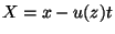 Eq. (26) becomes
and so  , i.e. the concentration is independent of time moving with
the local flow
, i.e. the concentration is independent of time moving with
the local flow  . Consider as in the previous section the case of an
instantaneous plane source at
. Consider as in the previous section the case of an
instantaneous plane source at  , . Then at
This must be the solution for all time, because
 .
Therefore
.
Therefore
Fig. 4. A line (or plane in 3-D) of pollutant
initially lying on is stretched and rotated by a shear flow .
At time the extent of the line of pollutant is denoted by  .
.
Consider the horizontal extent of the pollutant. At time it is
clearly
We can see that the pollutant spreads out at a rate proportional to . This
contrasts with the rate proportional to for diffusion, so it would
appear that advection is always more important than diffusion, except perhaps
for a short time after release. However, we shall see in the next section
that this is not the case.
2.3 Advection and Diffusion in a Shear Flow
When advection and diffusion occur simultaneously, the stretching of
regions of high concentration, as occurs for pure advection, is less
effective because transverse diffusion of the high concentration region is
enhanced by the stretching caused by the shear. This is shown schematically
in Fig. 5.
Fig. 5. An initial slab (a) of pollutant is rotated
and stretched by shear (b), leading to enhanced diffusion in the transverse
direction (c). The spreading of the line of maximum concentration is clearly
reduced by the diffusion.
The processes described here are known as Taylor's mechanism.
back to syllabus