10. Numerical Schemes
We will consider some finite difference numerical schemes for the
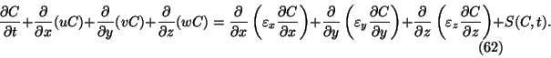
solution of the advection-diffusion equation with source term  :
:
10.1 Source Terms
The equation
can be approximated by
where  denotes
  evaluated at time
  . Eq. (64) is
not usually practical because stability is only achieved with severe
restrictions on the time step. Eq. (64) is an explicit scheme.
The corresponding implicit scheme is
. Eq. (64) is
not usually practical because stability is only achieved with severe
restrictions on the time step. Eq. (64) is an explicit scheme.
The corresponding implicit scheme is
This is unconditionally stable but if  is a nonlinear function,
Eq. (65) requires solution of a system of nonlinear equations.
Semi-implicit schemes are possible, such as
is a nonlinear function,
Eq. (65) requires solution of a system of nonlinear equations.
Semi-implicit schemes are possible, such as
If is a linear function, then the scheme (66) with  is
unconditionally stable and is furthermore second order accurate in
time, unlike (64) and (65) which are only first order accurate.
is
unconditionally stable and is furthermore second order accurate in
time, unlike (64) and (65) which are only first order accurate.
10.2 Advection Terms
Consider the simplified advection equation
where  is assumed to be constant. The simplest scheme is
where  denotes evaluated at
  and where
 . Eq. (68) is unconditionally unstable and
therefore useless. The Lax scheme is a modification of (68) in which
is replaced by
. Eq. (68) is unconditionally unstable and
therefore useless. The Lax scheme is a modification of (68) in which
is replaced by
 :
:
This scheme is stable if the Courant-Friedrichs-Lewy (CFL) condition
is satisfied. However, it is only first order accurate in time.
Another problem is that it is possible for to become negative.
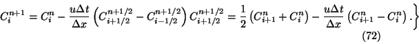
This problem is overcome in so-called upwind schemes:
This is stable if the CFL condition is satisfied but is only first
order accurate in space. Use of the upwind scheme is equivalent to the
introduction of a large artificial diffusion. A scheme which is
explicit, second order accurate in space and time and is stable if the
CFL condition is satisfied is the two-step Lax-Wendroff scheme:
This scheme does however still allow negative values of .
10.3 Diffusion Terms
Consider the simple, one-dimensional diffusion equation
For simplicity we will assume that the diffusivity  is constant.
An explicit scheme which is first order accurate in time and second
order accurate in space is
is constant.
An explicit scheme which is first order accurate in time and second
order accurate in space is
This is stable if
This usually requires a vast number of time steps for the effects of
diffusion to become noticeable. The fully implicit scheme
is unconditionally stable but it is necessary to solve a tridiagonal
system of equations at each time step. If the average of Eq. (74) and
(76) is taken we get the Crank-Nicholson scheme which is
unconditionally stable and second order accurate in space and time.
If is not constant, the above schemes can easily be
generalised. For example, we can write
10.4 Operator Splitting
For multi-dimensional problems or problems in which there is advection
and diffusion, many of the above methods can still be used if an
operator splitting approach is used. For example, consider the
one-dimensional advection-diffusion equation:
Now consider
By adding the first two equations in (79) we get Eq. (78) but we can
step forward these two equations separately, thus using the techniques
available for the solution of simpler equations.
As another example, consider the three-dimensional diffusion equation:
Using the notation in Eq. (77), we can solve
Adding these equations gives a consistent representation of
Eq. (80) which is second order accurate in space and time. This is an
alternating-direction implicit (ADI) method.
back to syllabus