1 Scalar Transport in the Atmosphere
1.1 Basic Principles
Consider an element of air containing a concentration  of a passive
pollutant (passive means that it doesn't react and is neutrally buoyant, i.e.
it doesn't settle).
of a passive
pollutant (passive means that it doesn't react and is neutrally buoyant, i.e.
it doesn't settle).
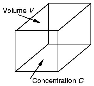
Fig 1. As an element of air is carried along by
the flow it always contains the same air and therefore contains the same
mass of pollutant.
If the flow is also incompressible, then the volume of the fluid element
remains constant and so the concentration remains constant. In mathematical
terms
It will be sufficient for our purposes to take the air to be incompressible
so that
Hence an alternative form of Eq. (1) is
Suppose now that there is a source or sink of the pollutant within the
element of air. This could be because the pollutant is created or destroyed
by chemical reactions or because there is an outflow from, say, a chimney.
The equation for would then become
where  represents the source term (in kgm
 s
s ). Examples could
be:
). Examples could
be:
(i)
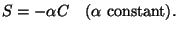 (5)
(5)
This represents decay of by, for example, chemical decomposition or
radioactive decay.
(ii)
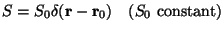 , (6)
, (6)
where
 is a delta function at
 .
This represents a continuous point source (e.g. emission from a chimney).
.
This represents a continuous point source (e.g. emission from a chimney).
(iii)
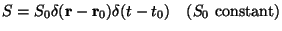 . (7)
. (7)
This represents an instantaneous point source occurring at time  at
(e.g. accidental release of a radioactive substance).
at
(e.g. accidental release of a radioactive substance).
Another type of source/sink term is caused by diffusion. The pollutant
may diffuse in or out of our element. The equation for is then
 is the molecular diffusivity. has dimensions
 .
Typical values for pollutants in the atmosphere are 5-50
.
Typical values for pollutants in the atmosphere are 5-50
 m
m s. We are usually concerned with dispersion on the scale of
hundreds of metres to hundreds of kilometres. Consider
s. We are usually concerned with dispersion on the scale of
hundreds of metres to hundreds of kilometres. Consider  m. Then
the time-scale is
m. Then
the time-scale is
which is infinite for all practical purposes. Hence molecular diffusion
is never directly relevant to atmospheric dispersion.
1.2 Turbulence
Atmospheric flows are almost always turbulent. Turbulence occurs when
the Reynolds number is high. It is characterised by eddy motions on a wide
range of scales. When describing the dispersion of pollutants, we are usually
interested in dispersion on scales much larger than many, if not all, of the
eddies. In other words, we are interested in averages over length or time
scales large compared to the turbulence.
In order to analyse dispersion in this way, we assume that it is possible to
divide the flow into a ``mean'' flow which is slowly varying in time and a
rapidly fluctuating, or ``turbulent'' part. We could perform this separation
by defining an average as follows:
The average period  should be chosen to be long compared to the turbulence
time-scales. Then we put
should be chosen to be long compared to the turbulence
time-scales. Then we put
 represents the turbulent part of
  . It follows (to a
reasonable approximation at least) that
. It follows (to a
reasonable approximation at least) that
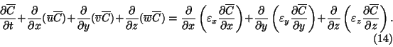
Let us perform this separation for all the variables in the concentration
equation, Eq. (3).
Therefore
We now average this equation. Consider, for example
since
 . Similar results hold for
  and
and  , giving
The right-hand side represents the average effect of turbulent eddies on the
concentration. Molecular diffusion is caused by the random motion of
molecules, whereas the effect here is caused by the random eddy motions. By
analogy with the molecular scale, we assume that
 ,
,
 and
and
 are analogous to the molecular diffusivity
. They must be measured experimentally. They differ from in that
(i)
,
and
need not be equal,
(ii) In general,
,
and
are not constant,
(iii)
are analogous to the molecular diffusivity
. They must be measured experimentally. They differ from in that
(i)
,
and
need not be equal,
(ii) In general,
,
and
are not constant,
(iii)
 .
.
Using Eq. (13),
This equation is the basis of much of the modelling of atmospheric dispersion.
back to syllabus